Introduction
fusion-blossom is a fast Minimum-Weight Perfect Matching (MWPM) solver for Quantum Error Correction (QEC).
Key Features
- Correctness: This is an exact MWPM solver, verified against the Blossom V library with millions of randomized test cases.
- Linear Complexity: The decoding time is roughly \( O(N) \) given small physical error rate, proportional to the number of defect vertices \( N \).
- Parallelism: A single MWPM decoding problem can be partitioned and solved in parallel, then fused together to find an exact global MWPM solution.
- Simple Interface: The graph problem is abstracted and optimized for QEC decoders.
Chapters
For beginners, please read how the MWPM decoder works and how we abstract the MWPM decoder interface in Problem Definition Chapter.
For experts in fusion-blossom, please jump to Installation or directly go to demos.
This library is written in Rust programming language for speed and memory safety, however, we do provide a Python package that expose commonly used functions.
Users can install the library using pip3 install fusion-blossom.
Contributing
fusion-blossom is free and open source. You can find the source code on GitHub, where you can report issues and request features using GitHub issue tracker. Currently the project is maintained by Yue Wu at Yale Efficient Computing Lab. If you'd like to contribute to the project, consider emailing the maintainer or opening a pull request.
License
The fusion-blossom library is released under the MIT License.
Problem Definition
We'll formally define the problem we're solving in this chapter.
We shall note that although fusion-blossom is a Minimum-Weight Perfect Matching (MWPM) solver, it only implicitly works on the complete graph where the MWPM problem is defined. In fact, our speed advantage originates from the sparse graph (decoding graph) we use that can implicitly yet accurately solve the problem on the complete graph (syndrome graph).
Decoding Graph vs. Syndrome Graph
The decoding graph \( (V_D, E_D) \) is naturally defined by the QEC code and the noise model. Every real vertex \( v \in V_D \) is a stabilizer measurement result. Every edge \( e = \langle u, v \rangle \in E_D \) corresponds to independent physical error(s) that can cause a pair of defect measurement results on vertices \( u, v \). Each edge has a non-negative weight \( w_e \), calculated by \( \ln \frac{1-p_e}{p_e} \) for the aggregated physical error rate \( p_e \le \frac{1}{2} \) (see explanation here). For open-boundary QEC codes, there are some errors that only generate a single defect measurement. We add some virtual vertices to the graph which is not a real stabilizer measurement but can be connected by such an edge.
Note that here we're assuming a single round of measurement. A normal stabilizer measurement means trivial measurement result (+1) and a defect stabilizer measurement means non-trivial measurement result (-1). This can be easily extended to multiple rounds of measurement, where a normal stabilizer measurement means the same result as the previous round, and a defect stabilizer stabilizer measurement means different result from the previous round.
The syndrome Graph \( (V_S, E_S) \) is generated from the decoding graph. In the syndrome graph, \( V_S \subseteq V_D \), where real vertices with normal measurement results are discarded, and only defect vertices and some virtual vertices are preserved. Syndrome graph first constructs a complete graph for the defect vertices, meaning there are edges between any pair of defect vertices. The weight of each edge in the syndrome graph \( e = \langle u_S, v_S \rangle \in E_S \) is calculated by finding the minimum-weight path between \( u_S, v_S \in V_D \) in the decoding graph. Apart from this complete graph, each vertex also connects to a virtual vertex if there exists a path towards any virtual vertex. For simplicity each real vertex only connects to one nearest virtual vertex.
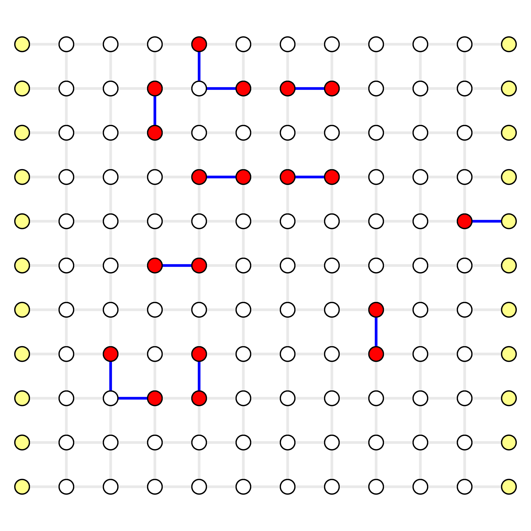
- white circle: real vertex \( v \in V_D, v \notin V_S \), a normal stabilizer measurement
- red circle: defect vertex \( v \in V_D, v \in V_S \), a defect stabilizer measurement
- yellow circle: virtual vertex \( v \in V_D \), non-existing stabilizer that is only used to support physical errors on the boundary of an open-boundary QEC code
- grey line: decoding graph edge \( e \in E_D \)
- pink line: syndrome graph edge \( e \in E_S \)
Decoding Graph
Syndrome Graph
On the syndrome graph, it's clear that it solves a Minimum-Weight Perfect Matching (MWPM) problem. A perfect matching is defined as a subset of edges \( M_S \subseteq E_S \) where each (real) vertex is incident by exactly one edge in \( M_S \). On the decoding graph, however, it's no longer a perfect matching. We name it as a Minimum-Weight Parity Subgraph (MWPS) problem. The syndrome pattern essentially sets a parity constraint on the result subgraph (or subset of edges \( M_D \subseteq E_D \)):
- Each real vertex is incident by edges in \( M_D \) with even times (even parity)
- Each defect vertex is incident by edges in \( M_D \) with odd times (odd parity)
- Each virtual vertex can be incident by arbitrary times (arbitrary parity)
Decoding Graph: Parity Subgraph
Syndrome Graph: Perfect Matching
We shall note that in a traditional MWPM decoder, people have to translate each matched pair in the minimum-weight perfect matching back to a chain of edges in the decoding graph. In fact, in order to use traditional MWPM libraries to implement a MWPM decoder, people translate from the decoding graph to the syndrome graph and then back to the decoding graph, which is not only time-consuming but also make the decoder implementation more complex. What we do here is to directly solve the problem on the decoding graph for high efficiency, and also directly output results on the decoding graph so that user can simply multiple the individual error for each edge to get the most-likely error pattern.
Our library can output both MWPS and MWPM. For more details, see Example QEC Codes. Here is an example in Python:
solver = SolverSerial(initializer)
solver.solve(syndrome)

# mwps: Vec<EdgeIndex>
mwps = solver.subgraph()  # preferred for simplicity

# mwpm: {
#     peer_matchings: Vec<(DefectIndex, DefectIndex)>,
#     virtual_matchings: Vec<(DefectIndex, VertexIndex)>,
# }
mwpm = solver.perfect_matching()  # traditional MWPM decoder output
How MWPM decoder works?
MWPM decoder essentially tries to find the most likely error pattern that generates a syndrome \( S \). Such an error pattern must satisfy the parity constrains to generate the given syndrome \( S \), either in the decoding graph (each defect vertex is incident by odd times) or in the syndrome graph (each vertex belongs to exactly one matching).
Suppose the aggregated probability for each edge is \( p_e \), independent from all other edges. An error pattern corresponds to a subset of edges \( E \), and the probability of this error pattern is
\[ \prod_{e \in E}{p_e} \prod_{e \notin E}{(1-p_e)} = \prod_{e \in E}{p_e} \prod_{e \in E}{\frac{1-p_e}{1-p_e}} \prod_{e \notin E}{(1-p_e)} = \prod_{e \in E}{\frac{p_e}{1-p_e}} \prod_{e}{(1-p_e)}\]
The last term \( \prod_{e}{(1-p_e)} \) is a constant, so maximizing the probability of an error pattern is equivalent to maximize the value of \( \prod_{e \in E}{\frac{p_e}{1-p_e}} \). We have
\[ \prod_{e \in E}{\frac{p_e}{1-p_e}} = \exp\left({\sum_{e \in E}{\ln \frac{p_e}{1-p_e}}}\right) = \exp\left({- \sum_{e \in E}{\ln \frac{1-p_e}{p_e}}}\right) \]
Given a reasonable error rate \( p_e \le \frac{1}{2} \), we have \( \frac{1-p_e}{p_e} \ge 1 \) and \( \ln \frac{1-p_e}{p_e} \ge 0 \). We assign weight to each edge as \( w_e = \ln \frac{1 - p_e}{p_e} \), a non-negative number. Thus, maximizing the probability of an error pattern is equivalent to minimizing the value while satisfying the parity constrains.
\[ \arg \min_{E} \sum_{e \in E} w_e = \arg \min_{E} \sum_{e \in E}{\ln \frac{1-p_e}{p_e}} \ \ \textrm{, subject to}\ S(E) = S \]
Installation
There are multiple ways to install this library. Choose any one of the methods below that best suit your needs.
Python Package
This is the easiest way to use the library. All the demos are in Python, but once you become familiar with the Python interface, the Rust native interface is exactly the same.
pip3 install fusion-blossom
Build from Source using Rust
This is the recommended way for experts to install the library, for two reasons. First, the pre-compiled binary doesn't include the Blossom V library due to incompatible license, and thus is not capable of running the verifier that invokes the blossom V library to double check the correctness of fusion blossom library. Second, you can access all the internal details of the library and reproduce the results in our paper.
Download the Blossom V Library [Optional]
Please note that you're responsible for requesting a proper license for the use of this library, as well as obeying any requirement.
In order to use the Blossom V algorithm as a verifier, you need to download the [kolmogorov2009blossom] library from https://pub.ist.ac.at/~vnk/software.html into the blossomV folder in the repository.
An example of downloading the Blossom V library is below. Note that the latest version number and website address may change over time.
wget -c https://pub.ist.ac.at/~vnk/software/blossom5-v2.05.src.tar.gz -O - | tar -xz
cp -r blossom5-v2.05.src/* blossomV/
rm -r blossom5-v2.05.src
You don't need to compile the Blossom V library manually.
Note that you can still compile the project without the Blossom V library. The build script automatically detects whether the Blossom V library exists and enables the feature accordingly.
Install the Rust Toolchain
We need the Rust toolchain to compile the project written in the Rust programming language. Please see https://rustup.rs/ for the latest instructions. An example on Unix-like operating systems is below.
curl --proto '=https' --tlsv1.2 -sSf https://sh.rustup.rs | sh
source ~/.bashrc  # this will add `~/.cargo/bin` to path
After installing the Rust toolchain successfully, you can compile the library and binary by
cargo build --release
cargo run --release -- test serial  # randomized test using blossom V as a verifier
Install the Python Development Tools [Optional]
If you want to develop the Python module, you need a few more tools
sudo apt install python3 python3-pip
pip3 install maturin
maturin develop  # build the Python package and install in your virtualenv or conda
python3 scripts/demo.py  # run a demo using the installed library
Install Frontend tools [Optional]
The frontend is a single-page application using Vue.js and Three.js frameworks.
To use the frontend, you need to start a local server.
Then visit http://localhost:8066/?filename=primal_module_serial_basic_10.json you should see a visualization of the solving process.
If you saw errors like fetch file error, then it means you haven't generated that visualization file.
Simply run cargo test primal_module_serial_basic_10 to generate the required file or run cargo test to generate all visualization files for the test cases.
python3 visualize/server.py
Install mdbook to build this tutorial [Optional]
In order to build this tutorial, you need to install mdbook and several plugins.
cargo install mdbook
cargo install mdbook-bib
cd tutorial
mdbook serve  # dev mode, automatically refresh the local web page on code change
mdbook build  # build deployment in /docs folder, to be recognized by GitHub Pages
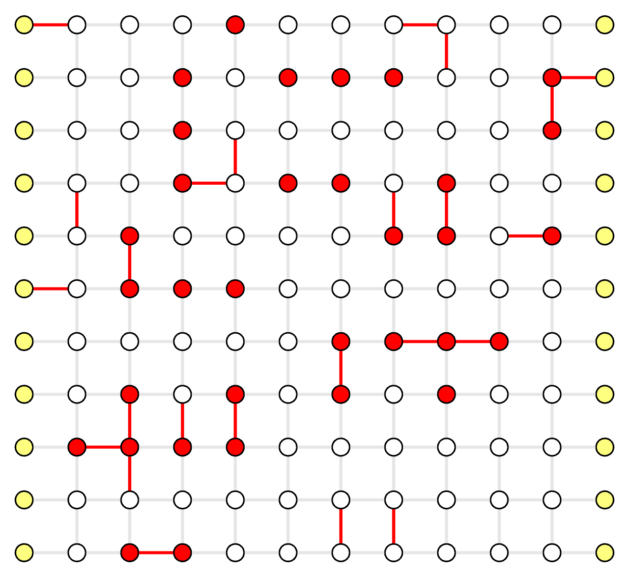
Example QEC Codes
In this chapter you'll learn how to use the builtin example QEC codes to run randomized decoder simulation and get familiar with the visualization tools.
You can download the complete code here.
Code Initialization
We provide several example QEC codes to demonstrate our solver. The code is defined by dimensions (usually code distance \( d \) and rounds of noisy measurement). The noise model is a simple i.i.d. noise model, given physical error rate \( p \).
import fusion_blossom as fb

code = fb.CodeCapacityPlanarCode(d=11, p=0.05, max_half_weight=500)
Current available QEC codes and noise models are:
CodeCapacityRepetitionCode(d, p)CodeCapacityPlanarCode(d, p)PhenomenologicalPlanarCode(d, noisy_measurements, p)CircuitLevelPlanarCode(d, noisy_measurements, p)
Simulate Random Errors
The example QEC code object can simulate random errors, outputs a syndrome pattern. You can provide a seed for the internal pseudo random number generator, otherwise it will use system-level random number for the seed. A syndrome pattern includes defect vertices (non-trivial stabilizer measurements) and also erasures (known-position errors, given by edge indices). Please check Construct Syndrome Chapter for more details of constructing your own syndrome.
syndrome = code.generate_random_errors(seed=1000)
print(syndrome)
An example output is: SyndromePattern { defect_vertices: [3, 14, 16, 17, 18, 26, 39, 40, 41, 42, 57, 62, 63, 79, 85, 87, 91, 98, 99], erasures: [] }
Initialize Visualizer [Optional]
visualizer = None
if True:  # change to False to disable visualizer for faster decoding
    visualize_filename = fb.static_visualize_data_filename()
    positions = code.get_positions()
    visualizer = fb.Visualizer(filepath=visualize_filename, positions=positions)
Initialize Solver
We use SolverSerial here as an example. Other solvers like SolverDualParallel and SolverParallel requires more input, please check Rust documentation for more information.
For the example QEC codes, we provide the initializer for the solver, but essentially it's a very simple format.
Please check Construct Decoding Graph Chapter for more details of constructing your own decoding graph initializer.
initializer = code.get_initializer()
solver = fb.SolverSerial(initializer)
Run Solver
The solver takes the syndrome as input and runs to a stable state. It also takes an optional parameter visualizer, to inspect the process of solving the problem.
solver.solve(syndrome)
Print Minimum-Weight Parity Subgraph (MWPS)
For definition of MWPS, please see Problem Definition Chapter.
The function subgraph() takes an optional visualizer object for visualization of the parity subgraph.
subgraph = solver.subgraph(visualizer)
print(f"Minimum Weight Parity Subgraph (MWPS): {subgraph}")
An example output is: Minimum Weight Parity Subgraph (MWPS): [14, 24, 26, 34, 66, 68, 93, 107, 144, 159, 161, 169]. Each number is an edge index, starting from 0 in the initializer.weighted_edges list. The visualization tool can help identify those edges (in blue).
Print Minimum-Weight Perfect Matching (MWPM)
For a traditional decoder implementation, it may want to take perfect matching as input. We also provide a method to get the minimum-weight perfect matching, grouped into two parts:
peer_matchings: Vec<(DefectIndex, DefectIndex)>: list of matched syndrome pairsvirtual_matchings: Vec<DefectIndex, VertexIndex>: list of syndrome matched to virtual vertices.
Note that type DefectIndex means the index applies to the syndrome list (usually used in a traditional decoder implementation).
In order to get the matched syndrome vertex indices, simply use the syndrome.defect_vertices list.
perfect_matching = solver.perfect_matching()
defect_vertices = syndrome.defect_vertices
print(f"Minimum Weight Perfect Matching (MWPM):")
print(f"    - peer_matchings: {perfect_matching.peer_matchings}")
peer_matching_vertices = [(defect_vertices[a], defect_vertices[b])
                            for a, b in perfect_matching.peer_matchings]
print(f"          = vertices: {peer_matching_vertices}")
virtual_matching_vertices = [(defect_vertices[a], b)
                            for a, b in perfect_matching.virtual_matchings]
print(f"    - virtual_matchings: {perfect_matching.virtual_matchings}")
print(f"             = vertices: {virtual_matching_vertices}")
Clear Solver
The solver is optimized to be repeatedly used, because the object construction is very expensive compared to solving the MWPS problem given usually a few defect vertices. The clear operation is a constant time operation.
solver.clear()
Visualization [Optional]
If you enabled the visualizer, then you can view it in your browser.
The Python package embeds the visualizer, so that you can view the visualizer output locally (by default to fb.static_visualize_data_filename() which is visualizer.json).
For more details about the visualizer and its usage, please refer to Visualizer Usage Chapter.
if visualizer is not None:
    fb.print_visualize_link(filename=visualize_filename)
    fb.helper.open_visualizer(visualize_filename, open_browser=True)
Construct Syndrome
In this chapter you'll learn how to construct your own syndrome to decode.
You can download the complete code here.
Code Initialization
We use a planar code as an example:
import fusion_blossom as fb

code = fb.CodeCapacityPlanarCode(d=11, p=0.05, max_half_weight=500)
Peek Graph [Optional]
If you want to customize the syndrome, it's easier to use the visualization tool to see which vertex you want to set to syndrome vertex. You can open it with:
fb.helper.peek_code(code) # comment out after constructing the syndrome
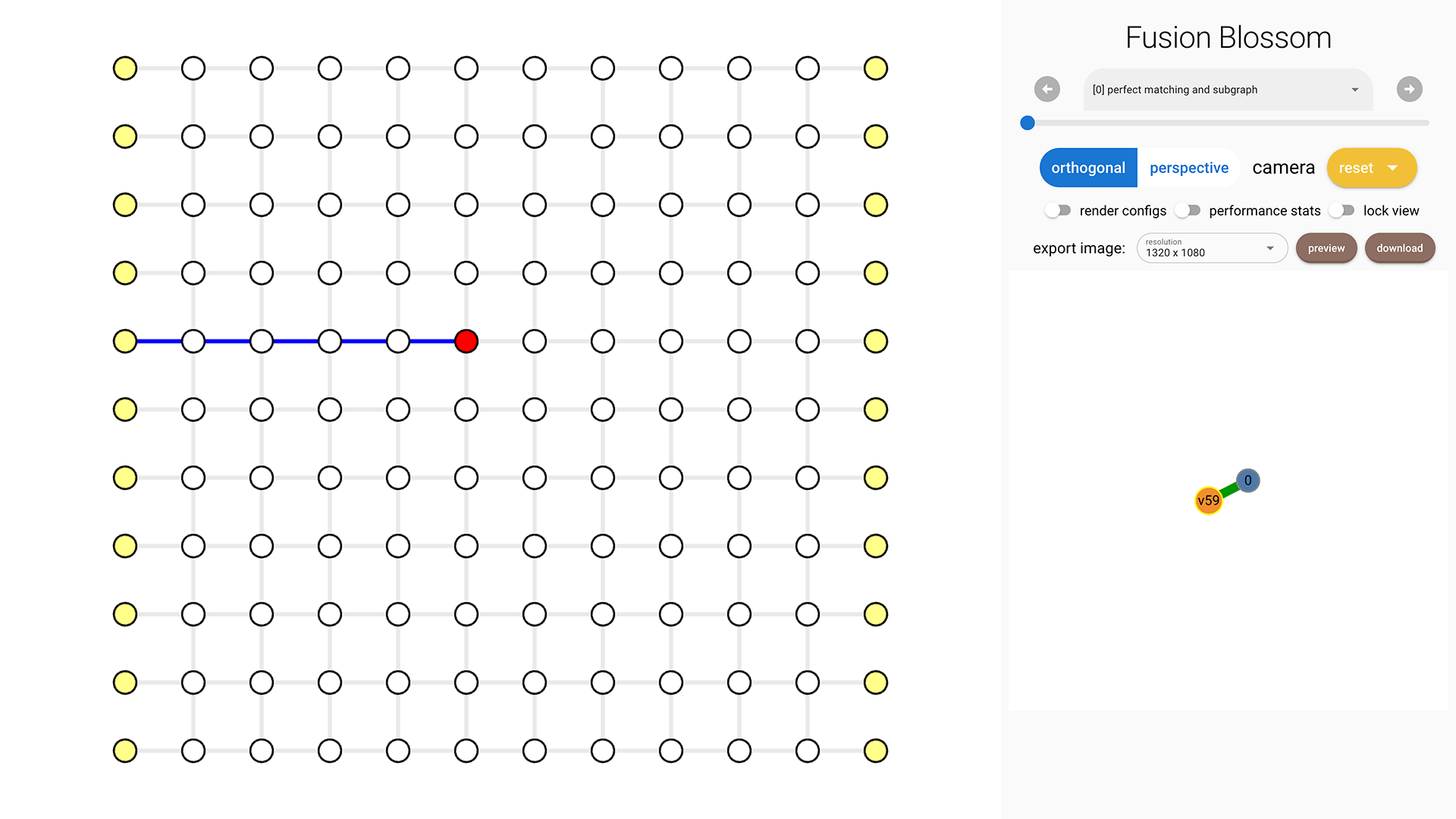
Click on each vertex to see its index on the right bottom. In this example, I'm selecting vertex 52.
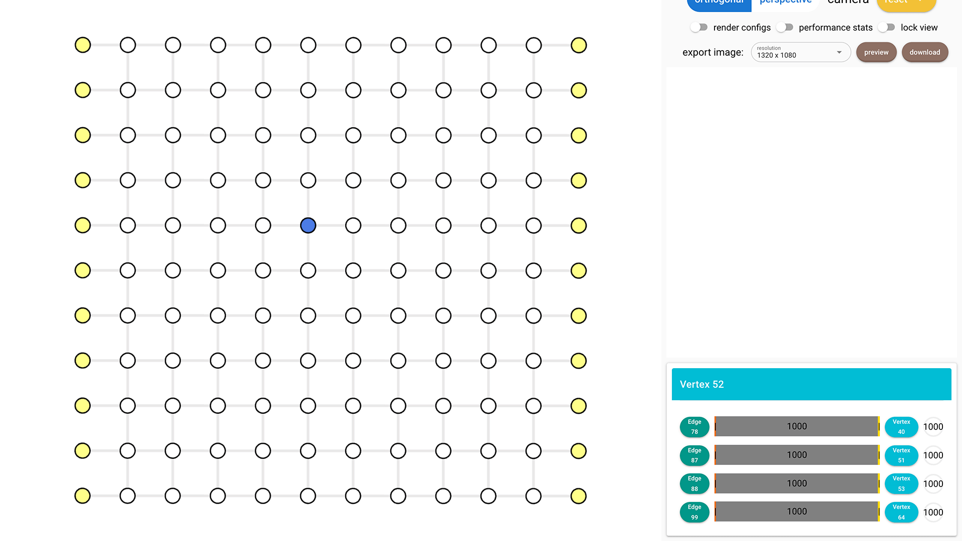
Construct Syndrome
A syndrome pattern takes 2 inputs: defect_vertices and erasures. They both default to empty list [].
We want to set vertex 52 as a syndrome vertex, so defect_vertices = [52].
A usual case for quantum error correction would have much less defect vertices than real vertices.
For more details about erasures, please see Decode Erasure Error Chapter.
syndrome = fb.SyndromePattern(
    defect_vertices = [52],
)
Visualize Result
The same process as in Example QEC Codes Chapter.
visualizer = None
if True:  # change to False to disable visualizer for faster decoding
    visualize_filename = fb.static_visualize_data_filename()
    positions = code.get_positions()
    visualizer = fb.Visualizer(filepath=visualize_filename, positions=positions)

initializer = code.get_initializer()
solver = fb.SolverSerial(initializer)

solver.solve(syndrome)

subgraph = solver.subgraph(visualizer)
print(f"Minimum Weight Parity Subgraph (MWPS): {subgraph}")  # Vec<EdgeIndex>

if visualizer is not None:
    fb.print_visualize_link(filename=visualize_filename)
    fb.helper.open_visualizer(visualize_filename, open_browser=True)
Construct Decoding Graph
In this chapter you'll learn how to construct your own decoding graph. Please make sure you understand everything about decoding graph in the Problem Definition Chapter.
You can download the complete code here.
Code Definition
We construct a customized repetition code with non-i.i.d. noise model.
That is, each qubit can have different probability of errors.
First we define a class representing this customized QEC code.
It must have two functions: get_positions and get_initializer.
We leave the detailed implementation of them to later part.
For the code itself, it takes a code distance \( d \) and a list of error rates \( \{ p_e \} \) specifying the error rate on each of the \( d \) data qubits.
import fusion_blossom as fb
import math

class CustomRepetitionCode:
    """A customize repetition code with non-i.i.d. noise model"""
    def __init__(self, d, p_vec):
        assert len(p_vec) == d
        self.d = d
        self.p_vec = p_vec
    def get_initializer(self):
        # missing implementation
    def get_positions(self):
        # missing implementation
Construct Initializer
There are \( d \) qubits in a chain, and the repetition code stabilizers exist in between every neighbor pair of qubits.
Thus, there are \( d-1 \) stabilizer qubits.
For simplicity we assume there are no measurement errors so we just need to decode a single round of measurement, which has \( d-1 \) real vertices.
Since the qubit on the left and right will generate a single non-trivial measurement event, a virtual vertex is added on the left and right respectively.
Thus, there are vertex_num = (d - 1) + 2 vertices in the decoding graph, in which the first and last are virtual vertices.
For the edges, we first calculate the weight using \( w_e = \ln \frac{1 - p_e}{p_e} \).
The fusion blossom algorithm takes even integer weight as input (which is also the default and recommended behavior in Blossom V library).
In order to minimize numerical error in the computation, we scale all the weight up to a maximum of 2 * max_half_weight.
class CustomRepetitionCode:
    def get_initializer(self, max_half_weight=500):
        vertex_num = (self.d - 1) + 2
        virtual_vertices = [0, vertex_num - 1]
        real_weights = [math.log((1 - pe) / pe, math.e) for pe in self.p_vec]
        scale = max_half_weight / max(real_weights)
        half_weights = [round(we * scale) for we in real_weights]
        weighted_edges = [(i, i+1, 2 * half_weights[i]) for i in range(vertex_num-1)]
        return fb.SolverInitializer(vertex_num, weighted_edges, virtual_vertices)
An example output for d = 7, p_vec = [1e-3, 0.01, 0.01, 0.01, 0.01, 1e-3, 1e-3] is
SolverInitializer {
    vertex_num: 8,
    weighted_edges: [(0, 1, 1000), (1, 2, 666), (2, 3, 666), (3, 4, 666)
        , (4, 5, 666), (5, 6, 1000), (6, 7, 1000)],
    virtual_vertices: [0, 7]
}
Construct Positions [Optional]
Positions are required only when you want to use the visualization tool. We just put all the vertices in a row in a equal space, although the actual weight of edges might be different.
class CustomRepetitionCode:
    def get_positions(self):
        return [fb.VisualizePosition(0, i, 0) for i in range(self.d + 1)]
Code Initialization
p_vec = [1e-3, 0.01, 0.01, 0.01, 0.01, 1e-3, 1e-3]
code = CustomRepetitionCode(d=len(p_vec), p_vec=p_vec)
Construct Syndrome
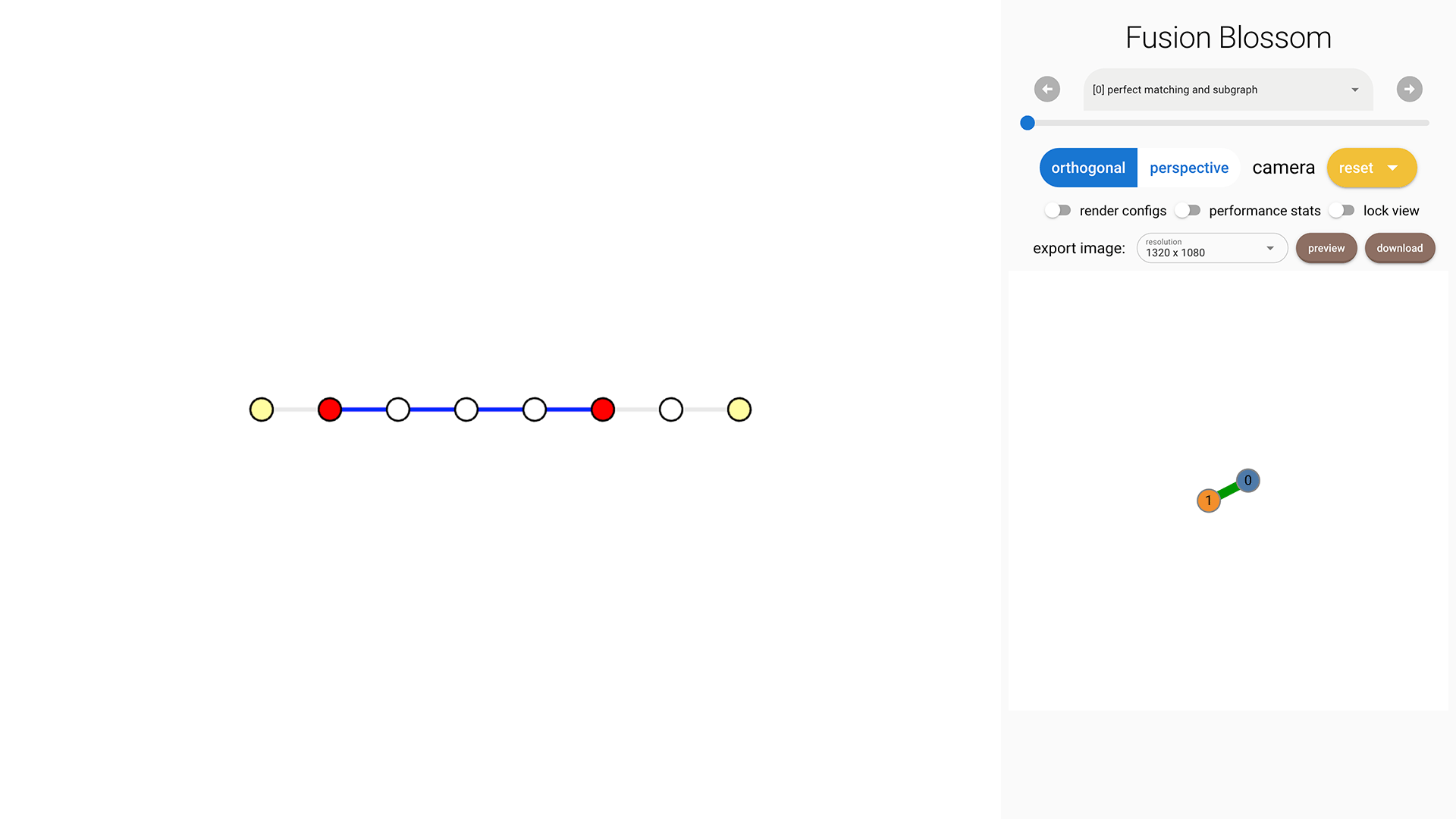
We use a syndrome pattern below to demonstrate the effect of weights.
syndrome = fb.SyndromePattern(defect_vertices=[1,5])
As shown in the following image, there are 4 edges selected in the Minimum-Weight Parity Subgraph (MWPS). This is because the weight sum of these 4 edges is 2664 but the sum of the other 3 complementary edges is 3000. This can also be explained by the fact that the probability is roughly \( 0.01^4 = 10^{-8} \) for the MWPS, but the complementary parity subgraph has a probability of roughly \( 0.001^3 = 10^{-9} \) which is less likely.
Visualize Result
The same process as in Example QEC Codes Chapter.
visualizer = None
if True:  # change to False to disable visualizer for faster decoding
    visualize_filename = fb.static_visualize_data_filename()
    positions = code.get_positions()
    visualizer = fb.Visualizer(filepath=visualize_filename, positions=positions)

initializer = code.get_initializer()
solver = fb.SolverSerial(initializer)

solver.solve(syndrome)

subgraph = solver.subgraph(visualizer)
print(f"Minimum Weight Parity Subgraph (MWPS): {subgraph}")  # Vec<EdgeIndex>

if visualizer is not None:
    fb.print_visualize_link(filename=visualize_filename)
    fb.helper.open_visualizer(visualize_filename, open_browser=True)
Use Results
In this chapter you'll learn how to use the MWPS results to construct the most likely error pattern.
You can download the complete code here.
Code Initialization
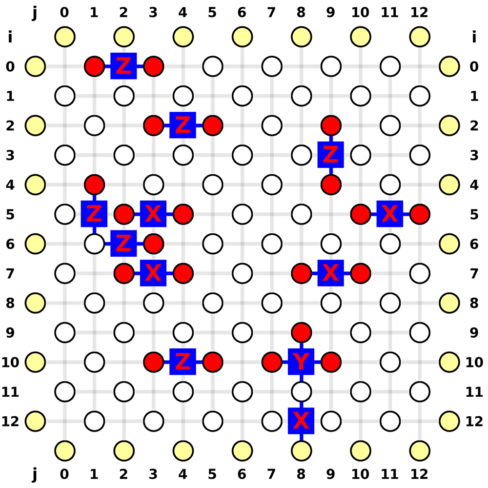
In a surface code with perfect measurement, we usually need to decode X stabilizers and Z stabilizers separately. The X stabilizers detect Pauli Z errors on data qubit, and Z stabilizers detect Pauli X errors on data qubit. For those more complex circuit-level noise model, it's similar but just some edges do not correspond to data qubit errors.
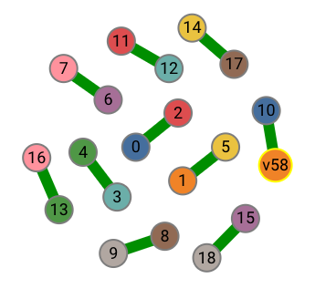
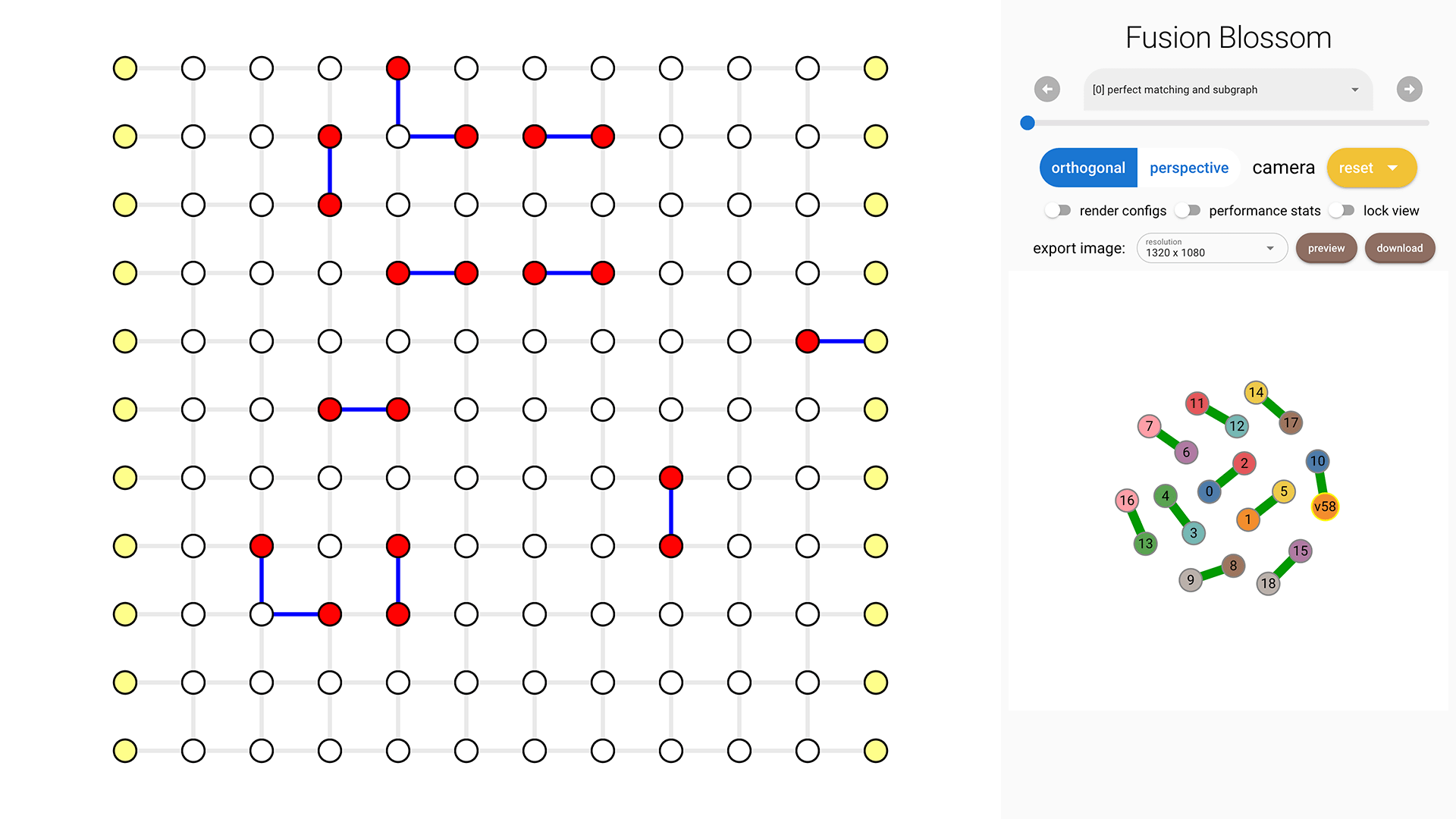
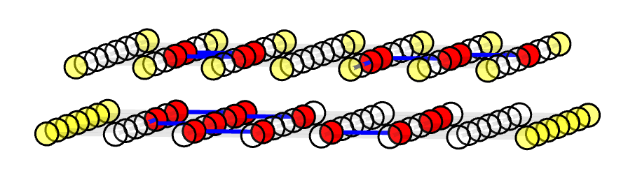
We first construct an example planar code. Note that this is only for either X stabilizer or Z stabilizer. It's perfectly fine to decode them separately, but in this case, I'll put both X and Z decoding graphs into a single decoding graph for better visual effect. They're still disconnected, as shown in the 3D plot here:
code = fb.CodeCapacityPlanarCode(d=7, p=0.1, max_half_weight=500)
Initialize Visualizer [Optional]
In order to plot them in a correct geometry, we swap the vertical i and horizontal j parameters for the the Z decoding graph.
We also place the Z decoding graph on top of the X decoding graph by setting t = 1, which do not affect the top view but can better distinguish X and Z decoding graphs if viewing in another direction (like the figure above).
visualizer = None
positions_x = code.get_positions()
positions_x = fb.center_positions(positions_x)
positions_z = [fb.VisualizePosition(pos.j, pos.i, 1) for pos in positions_x]
positions = positions_x + positions_z
if True:  # change to False to disable visualizer for faster decoding
    visualize_filename = fb.static_visualize_data_filename()
    visualizer = fb.Visualizer(filepath=visualize_filename, positions=positions)
Initialize Solver
We join the X and Z decoding graph. Note that this is not recommended for real applications but here we want to put X and Z decoding graph into a single graph for better visual.
initializer_x = code.get_initializer()
bias = initializer_x.vertex_num
weighted_edges_x = initializer_x.weighted_edges
virtual_vertices_x = initializer_x.virtual_vertices
weighted_edges_z = [(i + bias, j + bias, w) for (i, j, w) in weighted_edges_x]
virtual_vertices_z = [i + bias for i in virtual_vertices_x]
vertex_num = initializer_x.vertex_num * 2
weighted_edges = weighted_edges_x + weighted_edges_z
virtual_vertices = virtual_vertices_x + virtual_vertices_z
initializer = fb.SolverInitializer(vertex_num, weighted_edges, virtual_vertices)
solver = fb.SolverSerial(initializer)
Simulate Random Errors
We assume Pauli X and Pauli Z are independent error sources here for demonstration. Note that this is not depolarizing noise model. User should generate syndrome according to noise model instead of the graph itself.
syndrome_x = code.generate_random_errors(seed=1000)
syndrome_z = code.generate_random_errors(seed=2000)
defect_vertices = syndrome_x.defect_vertices
defect_vertices += [i + bias for i in syndrome_z.defect_vertices]
syndrome = fb.SyndromePattern(defect_vertices)
Visualize Result
The same process as in Example QEC Codes Chapter.
solver.solve(syndrome)

subgraph = solver.subgraph(visualizer)
print(f"Minimum Weight Parity Subgraph (MWPS): {subgraph}")  # Vec<EdgeIndex>

if visualizer is not None:
    fb.print_visualize_link(filename=visualize_filename)
    fb.helper.open_visualizer(visualize_filename, open_browser=True)
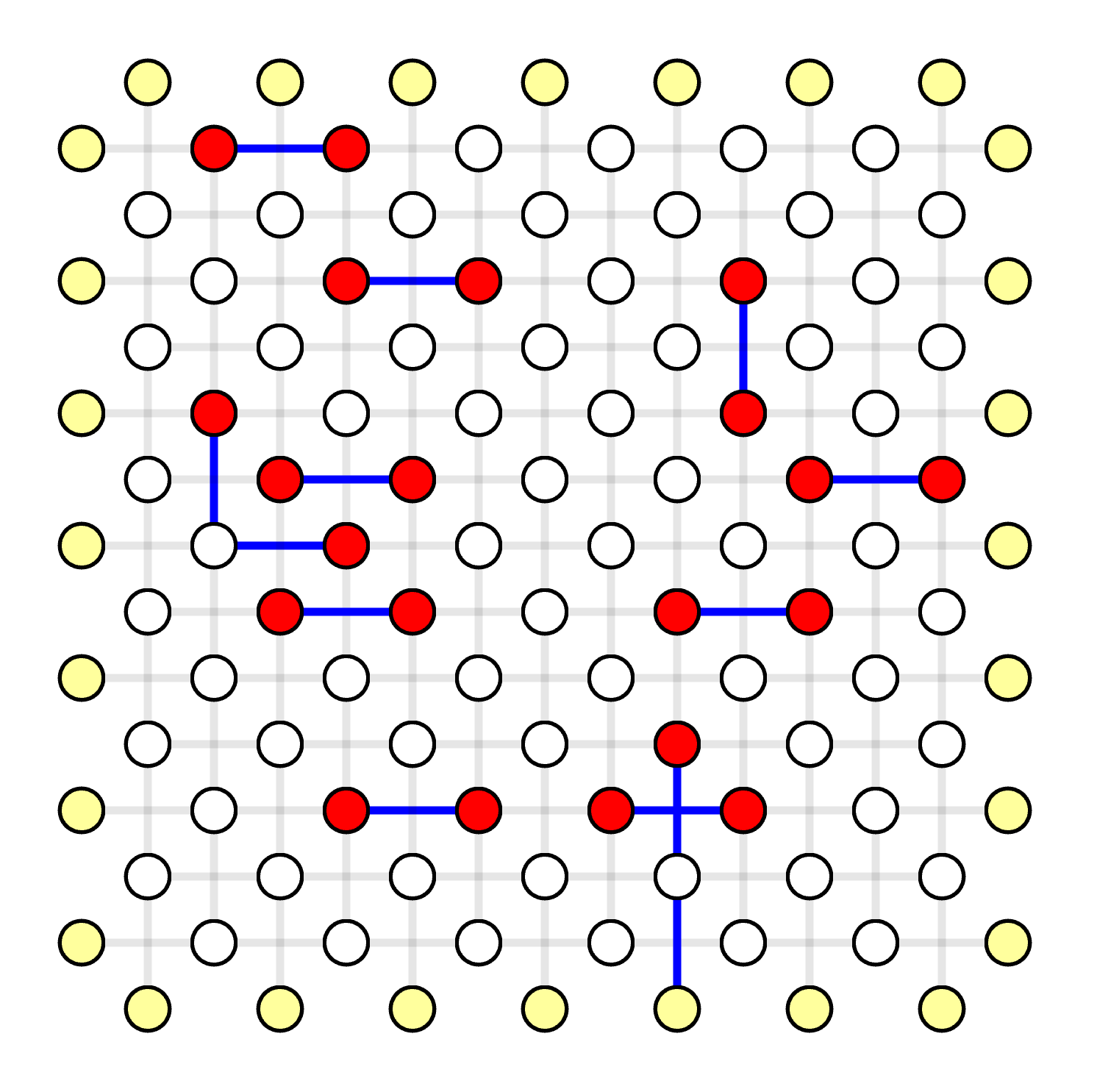
Generate Most Likely Error Pattern
Given the Minimum Weight Parity Subgraph (MWPS) is [0, 14, 24, 33, 39, 66, 68, 107, 108, 141, 142, 147, 159], now we need to construct the most likely error pattern as the result of MWPM decoder.
Here we use the position of qubit to identify qubits.
In real applications, one should record what are the corresponding physical errors for each edge when generating the decoding graph, so that it can query the error source for each edge.
error_pattern = dict()
for edge_index in subgraph:
    v1, v2, _ = weighted_edges[edge_index]
    qubit_i = round(positions[v1].i + positions[v2].i) + 6
    qubit_j = round(positions[v1].j + positions[v2].j) + 6
    error_type = "Z" if edge_index < len(weighted_edges_x) else "X"
    if (qubit_i, qubit_j) in error_pattern:
        error_pattern[(qubit_i, qubit_j)] = "Y"
    else:
        error_pattern[(qubit_i, qubit_j)] = error_type
print("Most Likely Error Pattern:", error_pattern)
An example output is
Most Likely Error Pattern: {
    (0, 2): 'Z',
    (2, 4): 'Z',
    (3, 9): 'Z',
    (5, 1): 'Z',
    (6, 2): 'Z',
    (10, 4): 'Z',
    (10, 8): 'Y',  # here is a Pauli Y error
    (5, 3): 'X',
    (7, 3): 'X',
    (12, 8): 'X',
    (7, 9): 'X',
    (5, 11): 'X'
}
The position indices and the most likely error pattern is marked below:
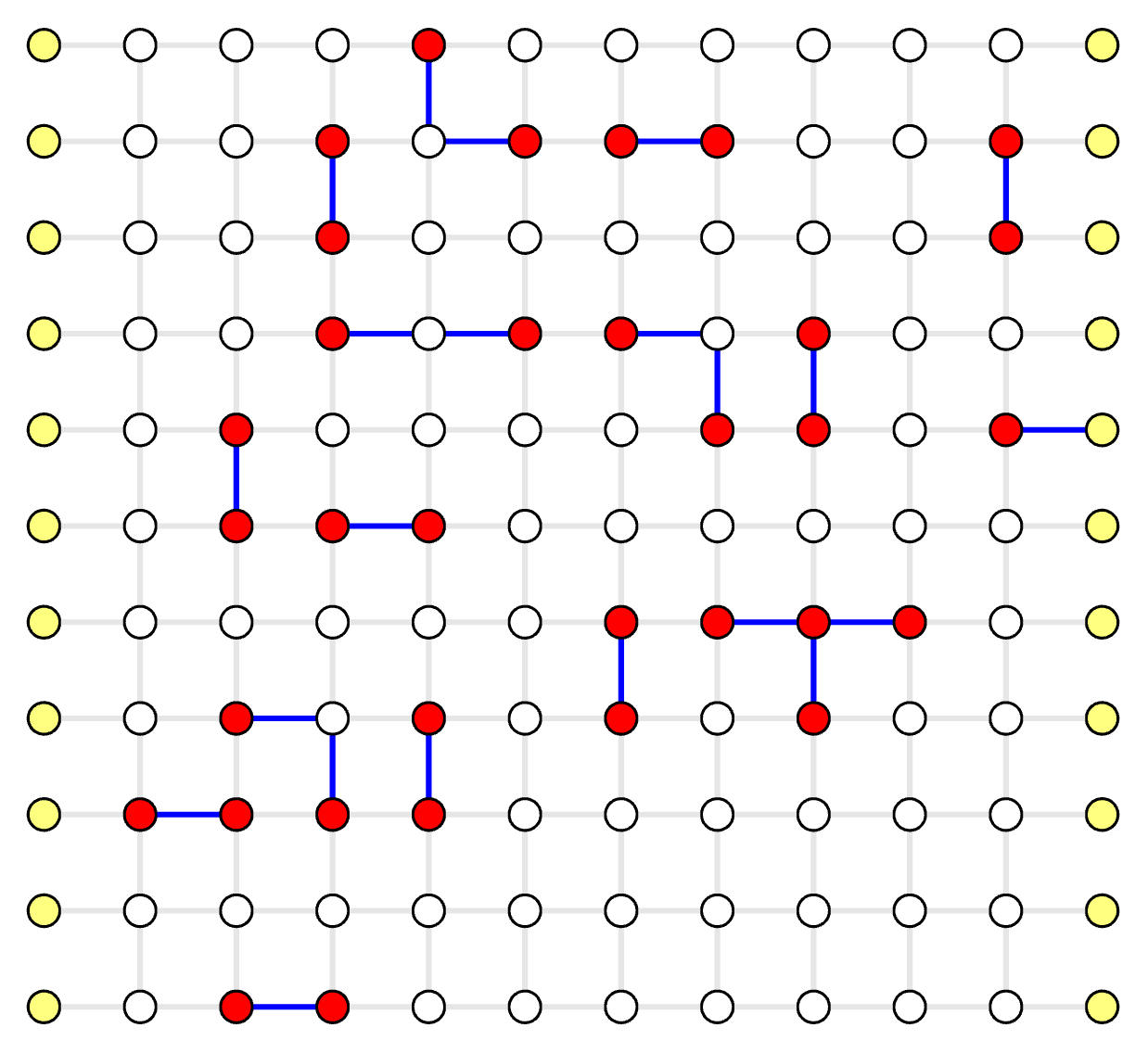
Decode Erasure Error
In this chapter you'll learn how to decode erasure errors, i.e. a known-position error.
You can download the complete code here.
Concepts
An erasure error is a known-position error where a qubit is replaced with a fresh qubit and can be modeled as going through error channel:
\[ \rho' = \frac{1}{4}(\rho + \hat{X}\rho\hat{X} + \hat{Y}\rho\hat{Y} + \hat{Z}\rho\hat{Z}) \]
Note that this kind of "loss" errors inherently exist, but knowing its position, aka erasure conversion, can help the decoder reach much higher accuracy than not using this position information. In the decoding graph, some of the edges must update their weights in order to utilize this position information. One way to do so is to set the weights of the corresponding edges to 0, because given a total loss \( p_e = \frac{1}{2} \), the weight is calculated by \( \ln\frac{1-p_e}{p_e} = 0 \). Fusion blossom library has native support for decoding erasure errors, by dynamically set some of the weights to 0.
Code Initialization
We use the erasure simulation in the example QEC codes. By setting the erasure probability, each edge is subject to erasure errors.
code = fb.CodeCapacityPlanarCode(d=11, p=0.05, max_half_weight=500)
code.set_erasure_probability(0.1)
Simulate Random Errors
syndrome = code.generate_random_errors(seed=1000)
print(syndrome)
An example output is
SyndromePattern {
    defect_vertices: [3, 14, 16, 17, 18, 21, 26, 33, 39, 40, 41, 54, 57, 62, 63
        , 79, 85, 87, 91, 96, 97, 98, 99, 121, 122],
    erasures: [10, 18, 41, 80, 92, 115, 159, 160, 161, 168, 180, 205, 206, 211]
}
You can also set the edge weights manually, using the following construction of a syndrome pattern:
fb.SyndromePattern(
    defect_vertices=[],  # Vec<VertexIndex)>
    erasures=[],         # Vec<EdgeIndex>, setting weights to 0
    dynamic_weights=[],   # Vec<(EdgeIndex, Weight)>, setting weights of certain edges to the new weights
)
The erasures are edge indices, whose weights will be set to 0 in the solver (red edges below).
Visualize Result
The same process as in Example QEC Codes Chapter.
Blossom Algorithm
Visualizer Usage
How to include image in README.md
The most elegant way I found is to follow this post: https://stackoverflow.com/a/42677655. At specific version, the image referred to is a fixed link.
To save Github build resources
The most expensive build action is for macOS: Your 2,420.00 included minutes used consists of 342.00 Ubuntu 2-core minutes, 328.00 Windows 2-core minutes, and 1,750.00 macOS 3-core minutes.
Since I'm using Mac for development already, I can run the following command to build it locally.
rustup target add x86_64-apple-darwin  # only once

CIBW_BUILD=cp38-* MACOSX_DEPLOYMENT_TARGET=10.12 CIBW_ARCHS_MACOS=universal2 python -m cibuildwheel --output-dir target