Example QEC Codes

In this chapter you'll learn how to use the builtin example QEC codes to run randomized decoder simulation and get familiar with the visualization tools.

You can download the complete code here.

Code Initialization

We provide several example QEC codes to demonstrate our solver. The code is defined by dimensions (usually code distance \( d \) and rounds of noisy measurement). The noise model is a simple i.i.d. noise model, given physical error rate \( p \).

import fusion_blossom as fb

code = fb.CodeCapacityPlanarCode(d=11, p=0.05, max_half_weight=500)

Current available QEC codes and noise models are:

CodeCapacityRepetitionCode(d, p)
CodeCapacityPlanarCode(d, p)
PhenomenologicalPlanarCode(d, noisy_measurements, p)
CircuitLevelPlanarCode(d, noisy_measurements, p)

Simulate Random Errors

The example QEC code object can simulate random errors, outputs a syndrome pattern. You can provide a seed for the internal pseudo random number generator, otherwise it will use system-level random number for the seed. A syndrome pattern includes defect vertices (non-trivial stabilizer measurements) and also erasures (known-position errors, given by edge indices). Please check Construct Syndrome Chapter for more details of constructing your own syndrome.

syndrome = code.generate_random_errors(seed=1000)
print(syndrome)

An example output is: SyndromePattern { defect_vertices: [3, 14, 16, 17, 18, 26, 39, 40, 41, 42, 57, 62, 63, 79, 85, 87, 91, 98, 99], erasures: [] }

Initialize Visualizer [Optional]

visualizer = None
if True:  # change to False to disable visualizer for faster decoding
    visualize_filename = fb.static_visualize_data_filename()
    positions = code.get_positions()
    visualizer = fb.Visualizer(filepath=visualize_filename, positions=positions)

Initialize Solver

We use SolverSerial here as an example. Other solvers like SolverDualParallel and SolverParallel requires more input, please check Rust documentation for more information. For the example QEC codes, we provide the initializer for the solver, but essentially it's a very simple format. Please check Construct Decoding Graph Chapter for more details of constructing your own decoding graph initializer.

initializer = code.get_initializer()
solver = fb.SolverSerial(initializer)

Run Solver

The solver takes the syndrome as input and runs to a stable state. It also takes an optional parameter visualizer, to inspect the process of solving the problem.

solver.solve(syndrome)

Print Minimum-Weight Parity Subgraph (MWPS)

For definition of MWPS, please see Problem Definition Chapter. The function subgraph() takes an optional visualizer object for visualization of the parity subgraph.

subgraph = solver.subgraph(visualizer)
print(f"Minimum Weight Parity Subgraph (MWPS): {subgraph}")

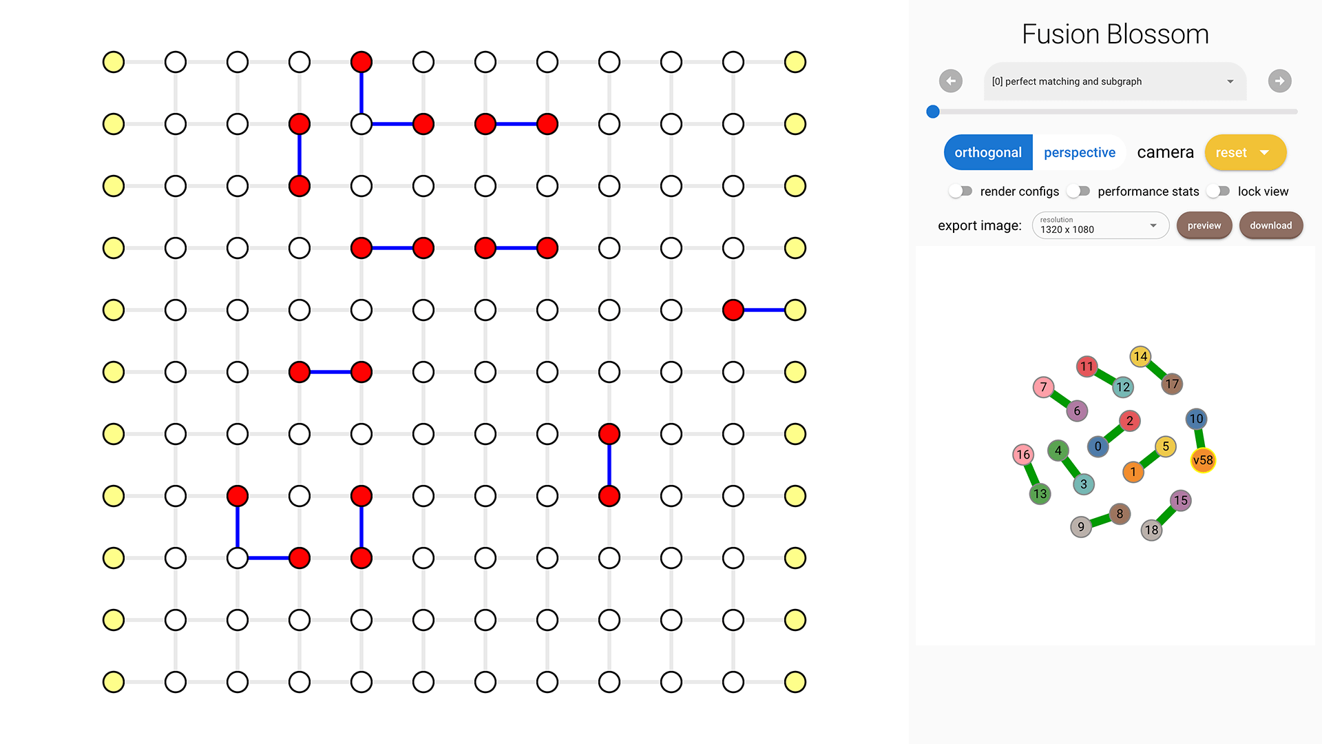
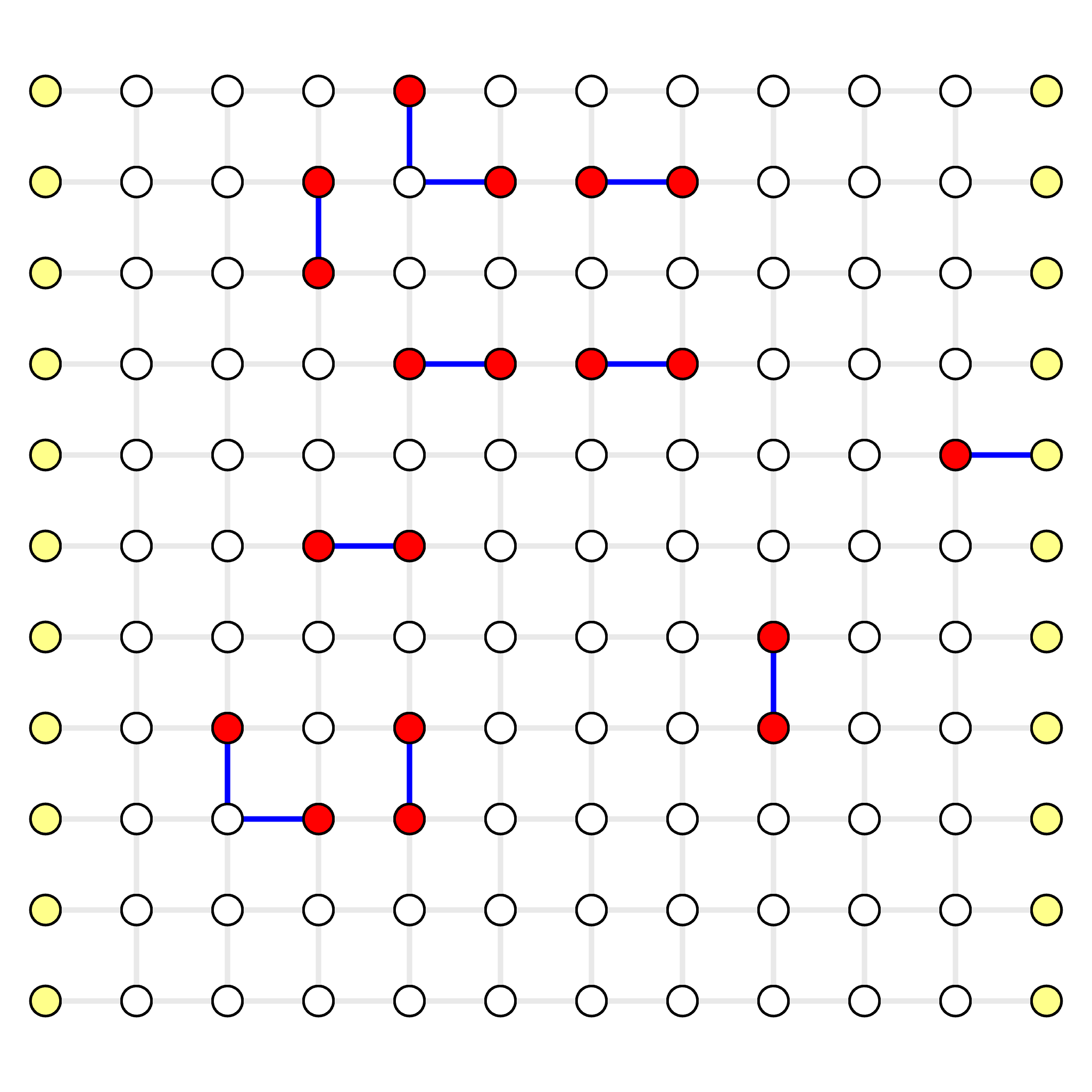
An example output is: Minimum Weight Parity Subgraph (MWPS): [14, 24, 26, 34, 66, 68, 93, 107, 144, 159, 161, 169]. Each number is an edge index, starting from 0 in the initializer.weighted_edges list. The visualization tool can help identify those edges (in blue).

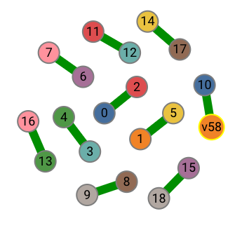
Print Minimum-Weight Perfect Matching (MWPM)

For a traditional decoder implementation, it may want to take perfect matching as input. We also provide a method to get the minimum-weight perfect matching, grouped into two parts:

peer_matchings: Vec<(SyndromeIndex, SyndromeIndex)>: list of matched syndrome pairs
virtual_matchings: Vec<SyndromeIndex, VertexIndex>: list of syndrome matched to virtual vertices.

Note that type SyndromeIndex means the index applies to the syndrome list (usually used in a traditional decoder implementation). In order to get the matched syndrome vertex indices, simply use the syndrome.defect_vertices list.

perfect_matching = solver.perfect_matching()
defect_vertices = syndrome.defect_vertices
print(f"Minimum Weight Perfect Matching (MWPM):")
print(f"    - peer_matchings: {perfect_matching.peer_matchings}")
peer_matching_vertices = [(defect_vertices[a], defect_vertices[b])
                            for a, b in perfect_matching.peer_matchings]
print(f"          = vertices: {peer_matching_vertices}")
virtual_matching_vertices = [(defect_vertices[a], b)
                            for a, b in perfect_matching.virtual_matchings]
print(f"    - virtual_matchings: {perfect_matching.virtual_matchings}")
print(f"             = vertices: {virtual_matching_vertices}")

Clear Solver

The solver is optimized to be repeatedly used, because the object construction is very expensive compared to solving the MWPS problem given usually a few defect vertices. The clear operation is a constant time operation.

solver.clear()

Visualization [Optional]

If you enabled the visualizer, then you can view it in your browser. The Python package embeds the visualizer, so that you can view the visualizer output locally (by default to fb.static_visualize_data_filename() which is visualizer.json). For more details about the visualizer and its usage, please refer to Visualizer Usage Chapter.

if visualizer is not None:
    fb.print_visualize_link(filename=visualize_filename)
    fb.helper.open_visualizer(visualize_filename, open_browser=True)

Fusion Blossom Tutorial